The P, the D and the Ugly

May 17, 2020 - lutz

2020 shall be the year when the 01. RFC Berlin wll be found. If it weren’t for COVID-19 this had already been done. Anyways, as the team’s name suggests it will be based in Berlin and if you don’t know “arm aber sexy” (poor but sexy) is the semi-official theme of the city. The lack of finance of the city is something we’ll experience too at the RFC so the plan is to reduce the costs of the robots as much as possible. In this post I want to tell about my adventures in making super cheap smart actuators.

The greatest matter of expense of the FUmanoid robots were the actuators: The FUmanoids employed Dynamixel actuators which are rather extortionately priced. Don’t get me wrong: You get plenty of actuator from the Dynamixels. Also they are quite hassle-free. But then, the actuators accounted for more than 90% of the overall costs (somewhere between 5k and 6k) of the robots. The RFC will be privately funded and there’s simply no way we could afford those actuators let alone an entire team of robots (with spares!).

The CIT Brains was the only team I remember that did not employ Dynamixel servos but rather RC servos as you’d use in model airplanes. Since the CIT Brains were pretty successful their actuator scheme cannot be a bad choice. So I set out to investigate if we could do something similar.

Here’s what I wish for in smart actuators:

• cheap
• easily available (preferably from multiple distributors)
• hackable (modifiable firmware)
• easy to replace/repair
• strong (comparable to the specs of the Dynamixels – which IMHO were rather optimistically stated in the documentations)

Yes, I am very aware of that list to be wishful thinking. Anyways, my idea was to buy cheapo-yet-strong RC Servos DS3218MG (about 16€ each) and replace the integrated electronics. I figured that a single Blue Pill (3€) in conjunction with three TB6612FNG (~5€ each) boards can drive up to six motors. As angular sensor I use AS5600 (12Bit absolute Hall encoders) on every joint which come at about 3.5€ per piece. The components total to 22.5€ per actuator which is super nice.

The DS3218MG is designed to work with up to 6V. However, more than 6V actually only grills the driver electronics that I’ve removed anyways. The motor that’s inside the servos can handle up to 6V according to it’s specification but my experiments showed that even 13V didn’t break them; even under load. Neat! If my math is correct this means that I could get twice the no-load speed and twice the holding torque out of the actuators! In theory that would be a whopping 4Nm for 22.5€!!!

Here’s how the no-load spinning of the motor looks like at 12V:

So I used some of my corona-at-home time to build a custom smart servo; or multiple actually.

There’s actually not that much to a smart servo apart from the control logic and and external interface. For the external interface I go with a custom USB device that can be interfaced with from a host via libusb. As for the control logic I wanted to try something new.

The Dynamixel motors have registers that you can read and write to. You can tell the servo to go to a certain position (angle/value/call-it-what-you-want) and to go there with a desired speed. The servo will then try it’s best to perform that action. However, I find the semantics behind this scheme a bit troubling.

There is a worst case movement that cannot be performed with the semantics of the dynamixel interface:

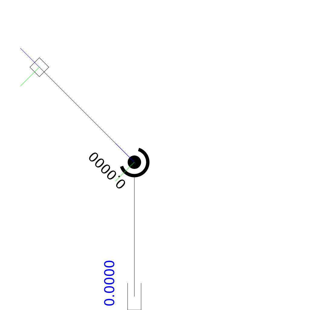
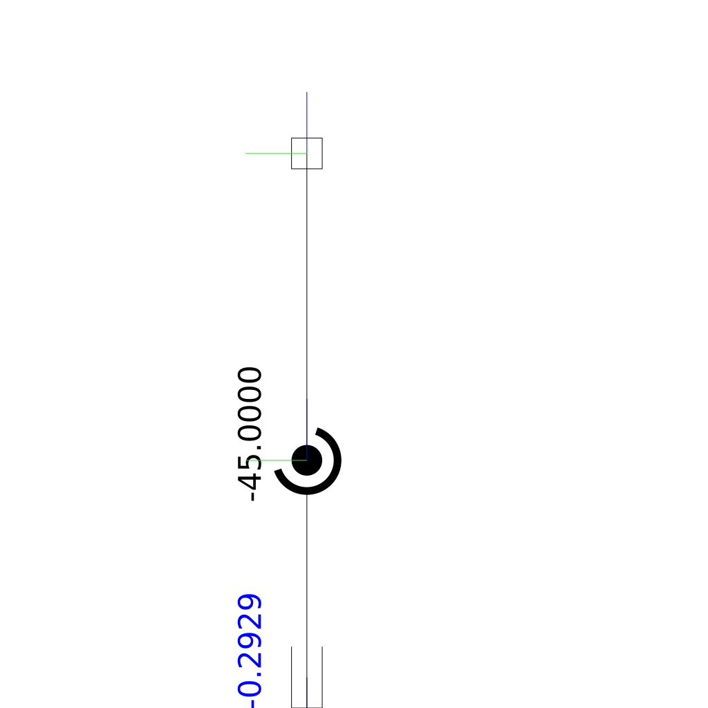
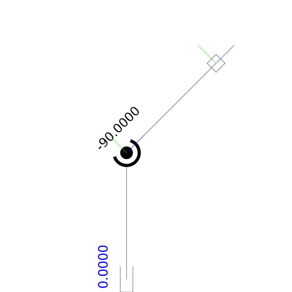
Consider the robot demonstrated above: The robot consists of a piston joint, a revolute joint and a finger. The Finger shall go from the left to the right along a straight line. The point is that when the motion starts as well when it ends the piston joint’s value is 0. When we’d apply the interface semantics of the dynamixel actuators we’d tell them at the beginning: go to position 0 with speed (say) -1$\frac{rad}{s}$. The Servo will happily comply and simply not move because it is already at the target position. In the next instant of time we’d tell the motor again to move to the position of 0 but with a slightly different speed. And again, the servo happily obliges by not moving at all. In the end the finger does not move along the line.

If you’ve read till here you’d maybe say that one could simply not calculate the final posture of a movement but a posture that is is the very near future. To you I shall respond: Yes, this would work around the issue but it does not solve it! I’d like to have it solved.

An alternative parameter set for servos

My solution to this problem is to change the semantics of how I tell the actuators to move: Instead of a goal value and a speed that shall be used to go to the target my actuators get a polynomial. The polynomial calculates the value for any given point in time. When this scheme is applied to the above scheme we’d tell the piston joint at the initial time step to move from position 0 with speed -1$\frac{rad}{s}$ (or whatever speed). This scheme also allows use of polynomials of higher degrees. Then the servo controller can also utilize information about acceleration to anticipate changes in the control behavior. Anyways, the coolest feature of those semantics is that it allows complex motion generation without intervention from the main control software.

At any given point in time the control software can calculate the posture and how the posture will time-locally evolve. The actuators take this information and execute it happily.

This leads to much smoother and more precise motion generation and the reduction of a lot of computations: Consider the classic interface semantics. To increase the smoothness of motion you’d need to increase the frequency of you telling the actuators how to move. With my scheme you don’t need to do it all that often. The deviation of the desired and actual motion increases much later in time.

Let’s talk about the P and the D

Here’s the part that actually deals with this post’s title: In virtually every actuator you’ll find some sort of PID controller.

In a nutshell a PID controller is a simple technique to calculate an output (force) given a target and a current value.

$u(t) = K_i * \int_{0}^{t} e(t) dt + K_p * e(t) + K_d * \frac{d e(t)}{dt}$

The formula consists of three parts:

• $K_i$: The integral part – This term counters constant external forces/disturbances.
• $K_p$: The proportional part – This term generates a force proportional to the current error.
• $K_d$: The derivative part – This dampens the output when the error changes (i.e., when the current value moves).

The $K_d$ part is of special interest to me as I’ve often implemented this part incorrectly. Also I’m very confident I’m not the only one implementing doing this mistake. To be fair when you read the wikipedia page about PID controlers non-zero target speeds are not exactly obvious.

My implementation reflected this term improperly: $\frac{d e(t)}{dt}$. I didn’t include the target speed! I just set this term equal to the negative of the current speed. What I unintentioally did was to assume the desired speed to be 0. With the above mentioned trajectory polynomial we now actually know the desired speed for any given t! And while we’re at it, we could also go a step further and extend the controller with another term for the second derivative:

$u(t) = K_i * \int_{0}^{t} e(t) dt + \sum_i K_i * (\frac{d^i v(t)}{d^i t} - \frac{d^i c(t)}{d^i t})$

The function $v(t)$ is the function of the target values over time, $c(t)$ is the value at time t. The term $\frac{d v(t)}{d t^i} - \frac{d c(t)}{d t^i}$ is the difference of the $i$-th derivative of the target and the $i$-th derivative of the current value by $t$. For $i=0$ this is the difference between the target and the current value, for $i=1$ it’s the difference between the target velocity and the current velocity and so on.

Neat. This reduces complexity! Unfortunately, the $K_i$ term cannot be generalized with this scheme.

Performance

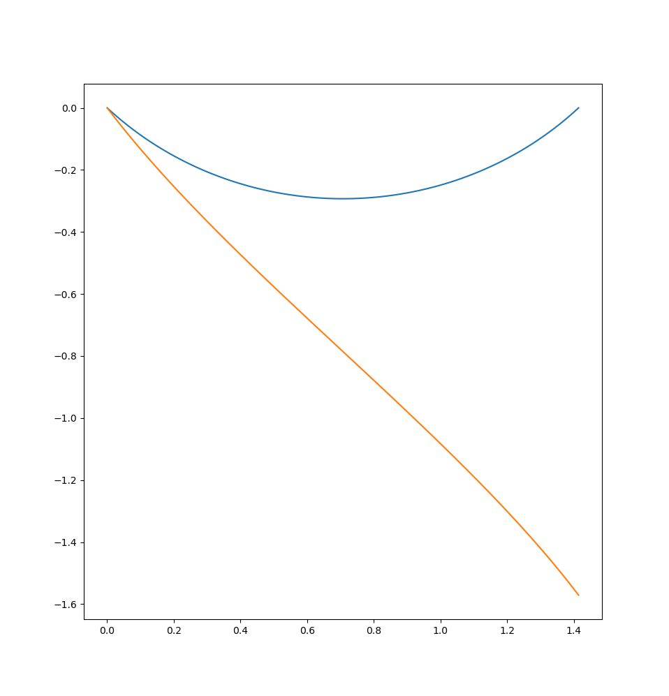
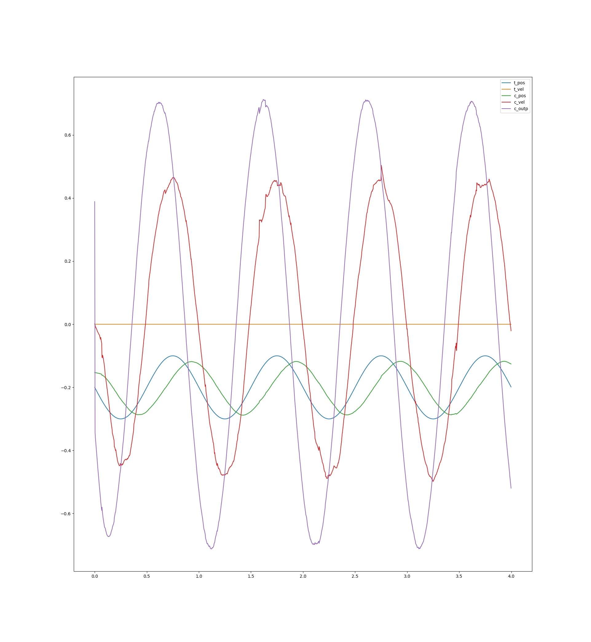
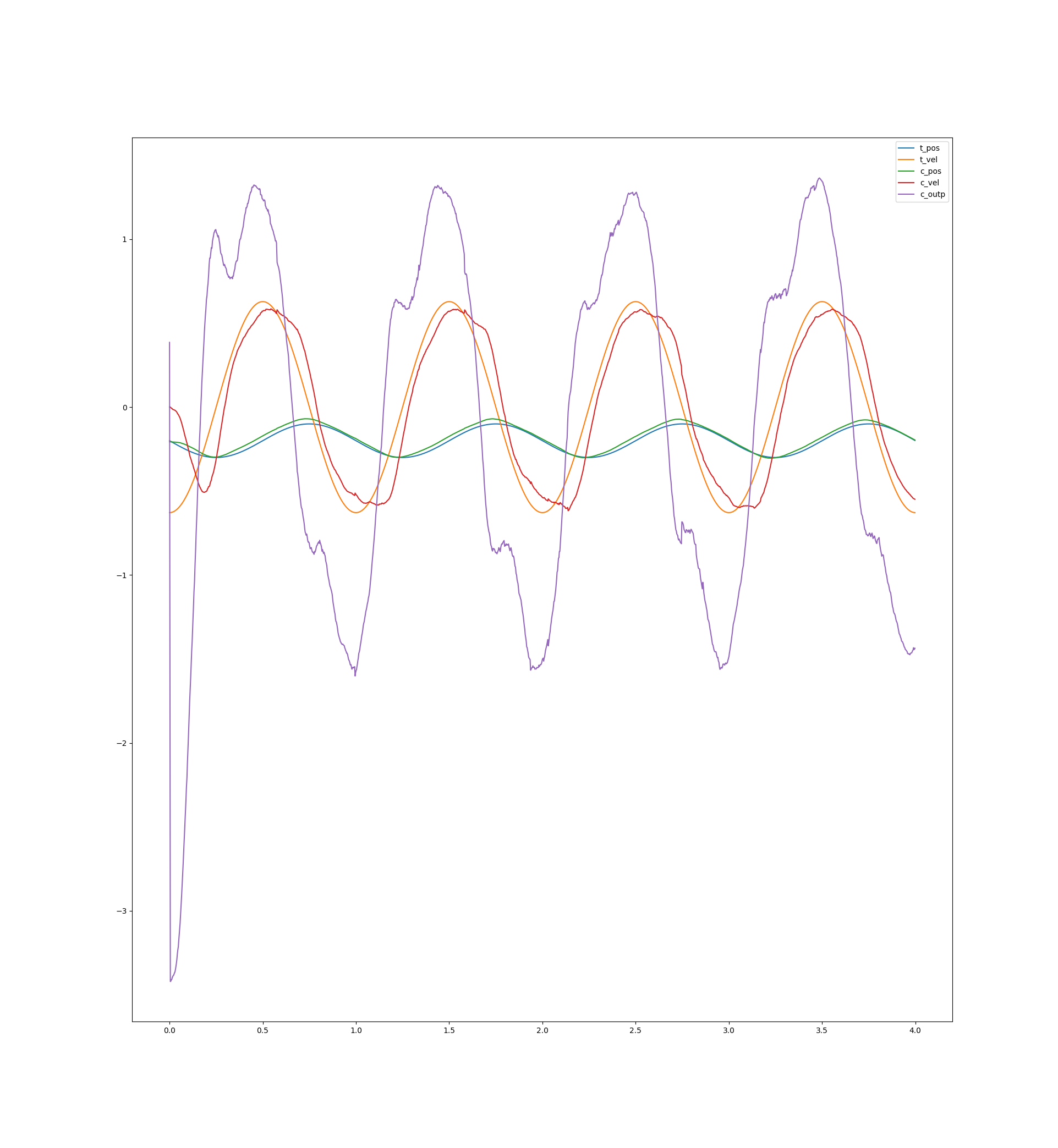
I’ve built a robot dog that utilizes the actuators and did some comparisons of the control behavior. The test was a sinusoidal movement of one of the dog’s knees with a velocity maximum of almost at the velocity limit. Here are the results:

Meanings of the colors:

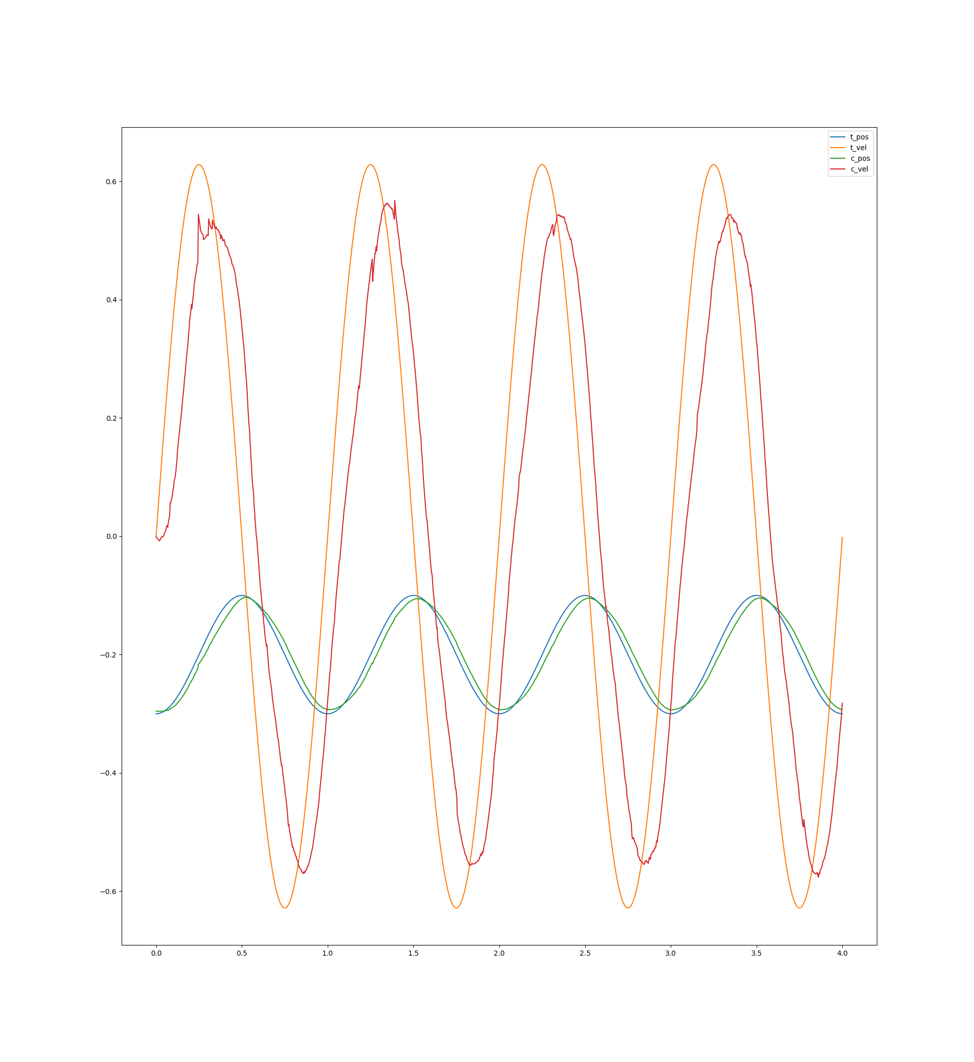
• blue: target value
• orange: target velocity
• green: current position
• red: current velocity (the velocity is a bit delayed due to a slow kalman filter that has to deal with high noise)
• violet: the output (only included in the first two plots)

Another neat trick is to account for the delay between sending the movement parameters and their application by applying a time offset when evaluating the trajectory polynomial:

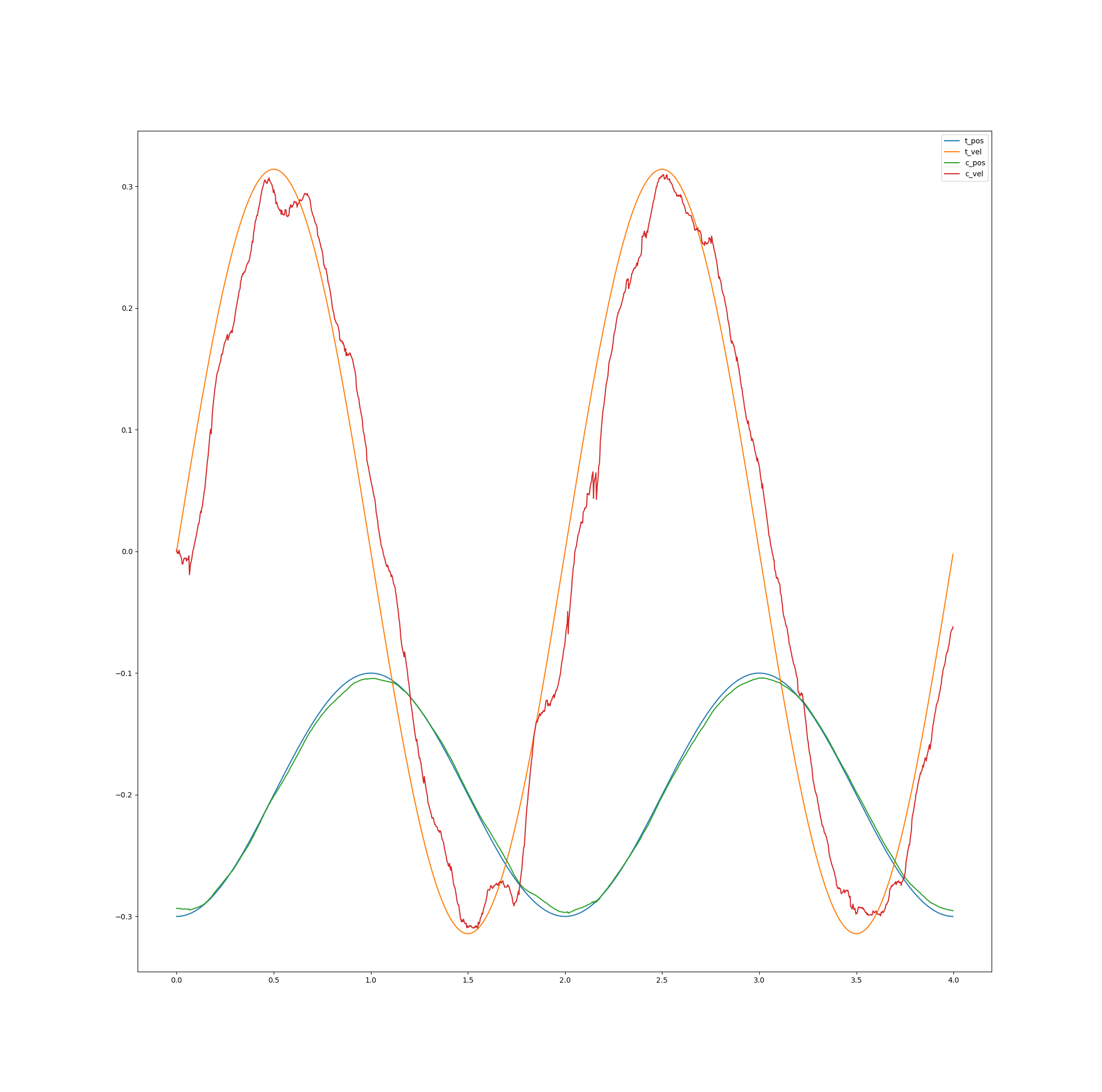
The maximum tracking error in the run of the last plot was below .005 (which is amounts to less than 2°). I’m biting my ass that I never did similar measurements with the dynamixel servos. But I’m very confident their tracking behavior was much worse.

TL;DR

You can build pretty decent actuators for very little money and while at it let them perform pretty damn well.